MATLAB - Идеальный фильтр нижних частот в обработке изображений
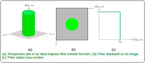
В области обработки изображений идеальный фильтр нижних частот (ILPF) используется для сглаживания изображения в частотной области. Он удаляет высокочастотный шум из цифрового изображения и сохраняет низкочастотные компоненты.
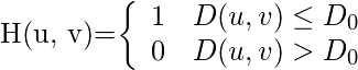
It can be specified by the function-
Where,
is a positive constant. ILPF passes all the frequencies within a circle of radius
This
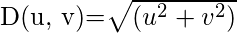
is the Euclidean Distance from any point (u, v) to the origin of the frequency plane, i.e,
Approach:
Step 1: Input – Read an image
Step 2: Saving the size of the input image in pixels
Step 3: Get the Fourier Transform of the input_image
Step 4: Assign the Cut-off Frequency
Step 5: Designing filter: Ideal Low Pass Filter
Step 6: Convolution between the Fourier Transformed input image and the filtering mask
Step 7: Take Inverse Fourier Transform of the convoluted image
Step 8: Display the resultant image as output
Implementation in MATLAB:
% MATLAB Code | Ideal Low Pass Filter % Reading input image : input_image input_image = imread("[name of input image file].[file format]"); % Saving the size of the input_image in pixels-% M : no of rows (height of the image)% N : no of columns (width of the image)[M, N] = size(input_image); % Getting Fourier Transform of the input_image% using MATLAB library function fft2 (2D fast fourier transform) FT_img = fft2(double(input_image)); % Assign Cut-off Frequency D0 = 30; % one can change this value accordingly % Designing filteru = 0:(M-1);idx = find(u>M/2);u(idx) = u(idx)-M;v = 0:(N-1);idy = find(v>N/2);v(idy) = v(idy)-N; % MATLAB library function meshgrid(v, u) returns% 2D grid which contains the coordinates of vectors% v and u. Matrix V with each row is a copy % of v, and matrix U with each column is a copy of u[V, U] = meshgrid(v, u); % Calculating Euclidean DistanceD = sqrt(U.^2+V.^2); % Comparing with the cut-off frequency and % determining the filtering maskH = double(D <= D0); % Convolution between the Fourier Transformed% image and the maskG = H.*FT_img; % Getting the resultant image by Inverse Fourier Transform% of the convoluted image using MATLAB library function % ifft2 (2D inverse fast fourier transform) output_image = real(ifft2(double(G))); % Displaying Input Image and Output Imagesubplot(2, 1, 1), imshow(input_image),subplot(2, 1, 2), imshow(output_image, [ ]); |
Input Image –
Output: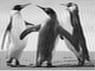

- Image-Processing
- MATLAB
- Advanced Computer Subject