Классификация данных с использованием опорных векторных машин (SVM) в R

В машинном обучении машина опорных векторов (SVM) - это модели обучения с учителем со связанными алгоритмами обучения, которые анализируют данные, используемые для классификации и регрессионного анализа. Он в основном используется в задачах классификации. В этом алгоритме каждый элемент данных отображается как точка в n-мерном пространстве (где n - количество функций), причем значение каждой функции является значением конкретной координаты. Затем выполняется классификация путем нахождения гиперплоскости, которая лучше всего различает два класса.

Помимо выполнения линейной классификации, SVM могут эффективно выполнять нелинейную классификацию, неявно отображая свои входные данные в пространственные объекты большой размерности.

Как работает SVM

Машина опорных векторов (SVM) - это дискриминантный классификатор, формально определяемый разделяющей гиперплоскостью. Другими словами, с учетом помеченных данных обучения (контролируемое обучение) алгоритм выводит оптимальную гиперплоскость, которая классифицирует новые примеры.

The most important question that arise while using SVM is how to decide right hyper plane. Consider the following scenarios:

• Scenario 1:
  In this scenario there are three hyper planes called A,B,C. Now the problem is to identify the right hyper-plane which best differentiates the stars and the circles.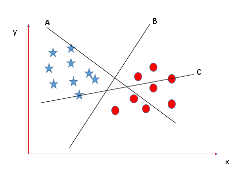

  

  The thumb rule to be known, before finding the right hyper plane, to classify star and circle is that the hyper plane should be selected which segregate two classes better.

  In this case B classify star and circle better, hence it is right hyper plane.

• Scenario 2:
  Now take another Scenario where all three planes are segregating classes well. Now the question arises how to identify the right plane in this situation.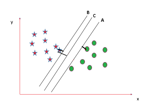

  

  In such scenarios, calculate the margin which is the distance between nearest data point and hyper-plane. The plane having the maximum distance will be considered as the right hyper plane to classify the classes better.

  Here C is having the maximum margin and hence it will be considered as right hyper plane.

Above are some scenario to identify the right hyper-plane.

Note: For details on Classifying using SVM in Python, refer Classifying data using Support Vector Machines(SVMs) in Python

Implementation of SVM in R

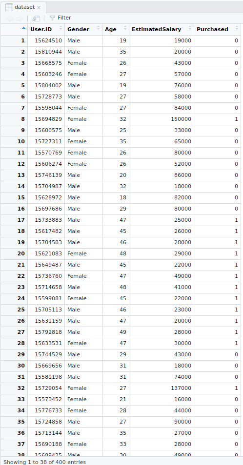
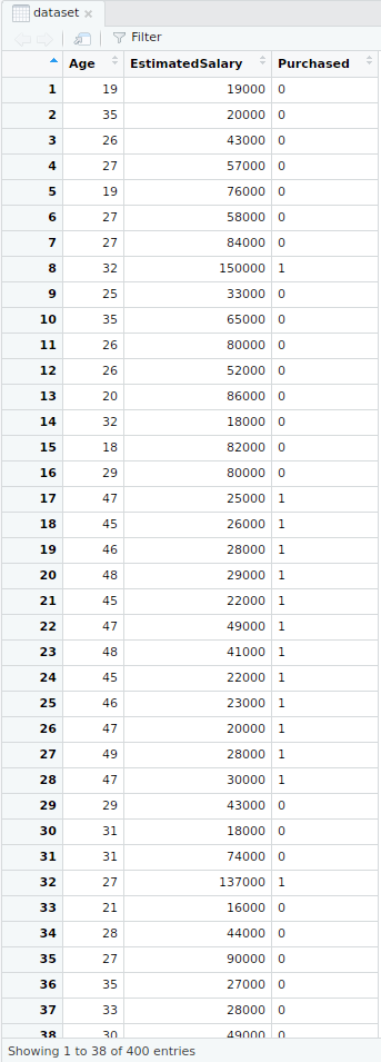
Here, an example is taken by importing a dataset of Social network aids from file Social.csv

The implementation is explained in the following steps:

• Importing the dataset

  # Importing the dataset dataset = read.csv("Social_Network_Ads.csv") dataset = dataset[3:5]

  Output:

  

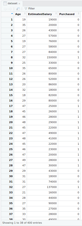
• Selecting columns 3-5
  This is done for the ease of computation and implementation (to keep the example simple).

  # Taking columns 3-5 dataset = dataset[3:5]

  Output:
  

• Encoding the target feature

  # Encoding the target feature as factor dataset$Purchased = factor(dataset$Purchased, levels = c(0, 1))

  Output:

  

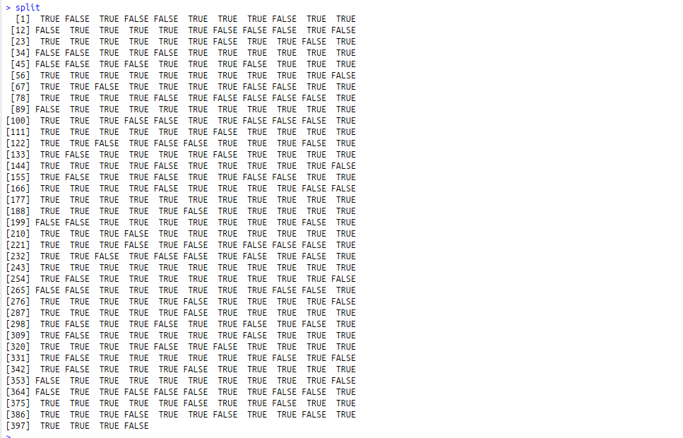
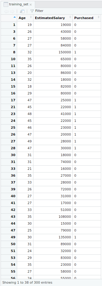
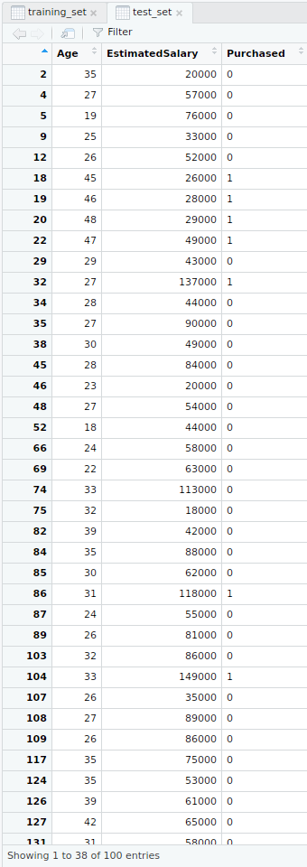
• Splitting the dataset

  # Splitting the dataset into the Training set and Test set install.packages("caTools") library(caTools)    set.seed(123) split = sample.split(dataset$Purchased, SplitRatio = 0.75)    training_set = subset(dataset, split == TRUE) test_set = subset(dataset, split == FALSE)

  Output:

  • Splitter

    

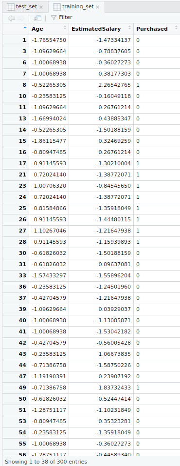
  • Training dataset

    

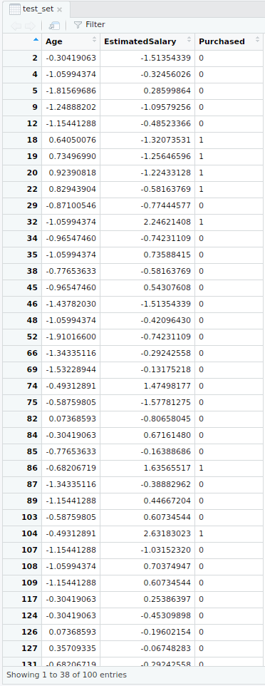
  • Test dataset

    

• Feature Scaling

  # Feature Scaling training_set[-3] = scale(training_set[-3]) test_set[-3] = scale(test_set[-3])

  Output:

  • Feature scaled training dataset

    

  • Feature scaled test dataset

    

• Fitting SVM to the training set

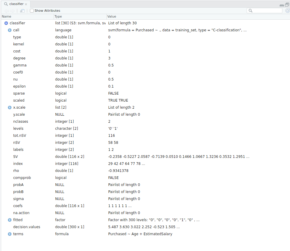
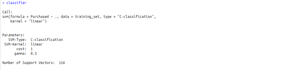
  # Fitting SVM to the Training set install.packages("e1071") library(e1071)    classifier = svm(formula = Purchased ~ .,                  data = training_set,                  type = "C-classification",                  kernel = "linear")

  Output:

  • Classifier detailed

    

  • Classifier in nutshell

    

• Predicting the test set result

  # Predicting the Test set results y_pred = predict(classifier, newdata = test_set[-3])

  Output:

  

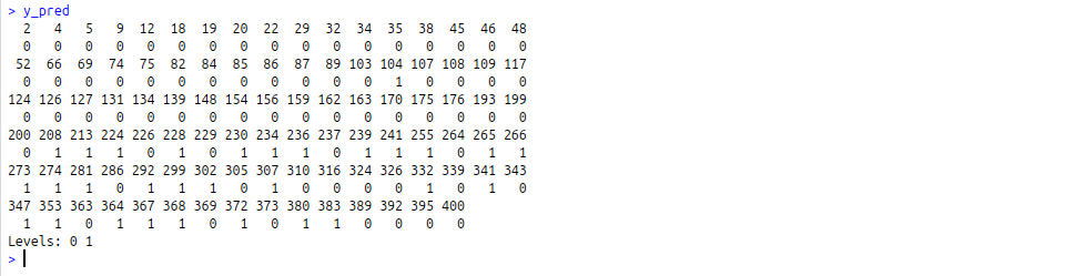
• Making Confusion Matrix

  # Making the Confusion Matrix cm = table(test_set[, 3], y_pred)

  Output:

  

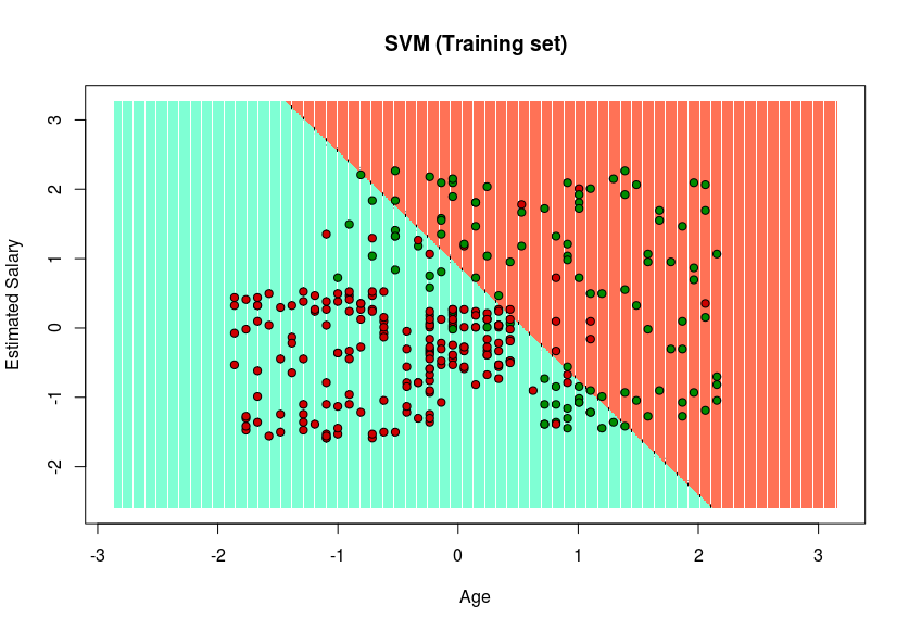
• Visualizing the Training set results

  # installing library ElemStatLearn library(ElemStatLearn)    # Plotting the training data set results set = training_set X1 = seq(min(set[, 1]) - 1, max(set[, 1]) + 1, by = 0.01) X2 = seq(min(set[, 2]) - 1, max(set[, 2]) + 1, by = 0.01)    grid_set = expand.grid(X1, X2) colnames(grid_set) = c("Age", "EstimatedSalary") y_grid = predict(classifier, newdata = grid_set)    plot(set[, -3],      main = "SVM (Training set)",      xlab = "Age", ylab = "Estimated Salary",      xlim = range(X1), ylim = range(X2))    contour(X1, X2, matrix(as.numeric(y_grid), length(X1), length(X2)), add = TRUE)    points(grid_set, pch = ".", col = ifelse(y_grid == 1, "coral1", "aquamarine"))    points(set, pch = 21, bg = ifelse(set[, 3] == 1, "green4", "red3"))

  Output:

  

• Visualizing the Test set results

  set = test_set X1 = seq(min(set[, 1]) - 1, max(set[, 1]) + 1, by = 0.01) X2 = seq(min(set[, 2]) - 1, max(set[, 2]) + 1, by = 0.01)    grid_set = expand.grid(X1, X2) colnames(grid_set) = c("Age", "EstimatedSalary") y_grid = predict(classifier, newdata = grid_set)    plot(set[, -3], main = "SVM (Test set)",      xlab = "Age", ylab = "Estimated Salary",      xlim = range(X1), ylim = range(X2))    contour(X1, X2, matrix(as.numeric(y_grid), length(X1), length(X2)), add = TRUE)    points(grid_set, pch = ".", col = ifelse(y_grid == 1, "coral1", "aquamarine"))    points(set, pch = 21, bg = ifelse(set[, 3] == 1, "green4", "red3"))

  Output:

  

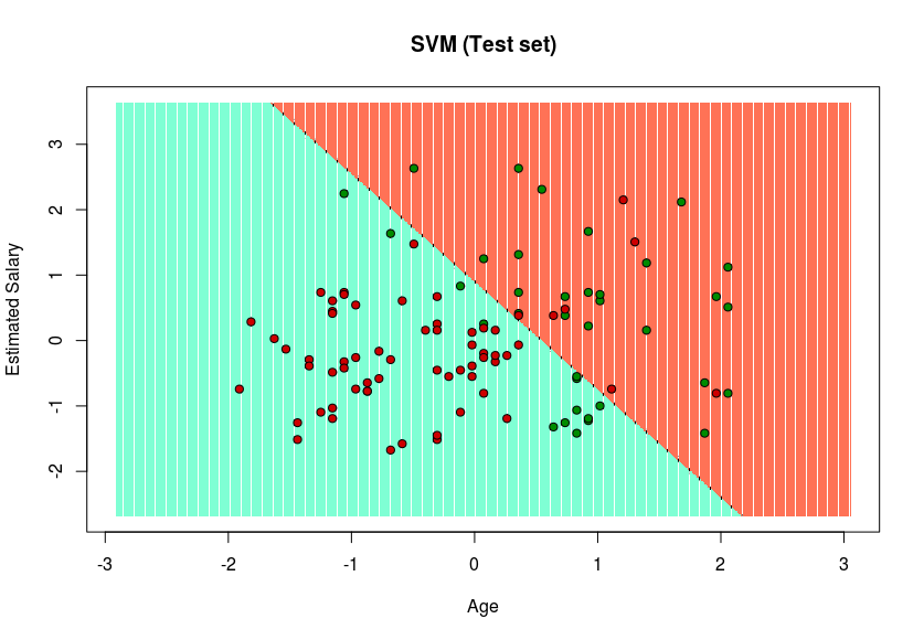
Since in the result, a hyper-plane has been found in the Training set result and verified to be the best one in the Test set result. Hence, SVM has been successfully implemented in R.