Регрессия и ее типы в программировании на R

Опубликовано: 31 Января, 2022

Регрессионный анализ - это статистический инструмент для оценки взаимосвязи между двумя или более переменными. Всегда есть одна переменная ответа и одна или несколько переменных-предикторов. Регрессионный анализ широко используется для соответствующей подгонки данных и последующего прогнозирования данных для прогнозирования. Это помогает предприятиям и организациям узнать о поведении своего продукта на рынке, используя переменную зависимую / ответную и независимую / предикторную переменную. В этой статье давайте узнаем о различных типах регрессии в программировании на R с помощью примеров.

Типы регрессии

В программировании R широко используются три основных типа регрессии. Они есть:

Линейная регрессия
Множественная регрессия
Логистическая регрессия

Линейная регрессия

Модель линейной регрессии - одна из наиболее широко используемых среди трех типов регрессии. В линейной регрессии взаимосвязь оценивается между двумя переменными, т. Е. Одной переменной ответа и одной переменной-предиктором. Линейная регрессия дает прямую линию на графике. Математически,

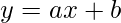
where,
x indicates predictor or independent variable
y indicates response or dependent variable
a and b are coefficients

Реализация в R

In R programming, lm() function is used to create linear regression model.

Syntax:
lm(formula)
Parameter:
formula: represents the formula on which data has to be fitted
To know about more optional parameters, use below command in console: help(“lm”)

Example:
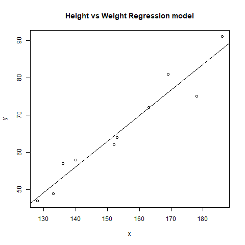
In this example, let us plot the linear regression line on the graph and predict the weight based using height.

# R program to illustrate
# Linear Regression
  
# Height vector
x <- c(153, 169, 140, 186, 128,
       136, 178, 163, 152, 133)
  
# Weight vector
y <- c(64, 81, 58, 91, 47, 57,
       75, 72, 62, 49)
  
# Create a linear regression model
model <- lm(y~x)
  
# Print regression model
print(model)
  
# Find the weight of a person 
# With height 182
df <- data.frame(x = 182)
res <-  predict(model, df)
cat("
Predicted value of a person 
               with height = 182")
print(res)
  
# Output to be present as PNG file
png(file = "linearRegGFG.png")
  
# Plot
plot(x, y, main = "Height vs Weight
                 Regression model")
abline(lm(y~x))
  
# Save the file.
dev.off()

Выход:

Вызов:
lm (формула = y ~ x)

Коэффициенты:
(Перехват) x  
   -39,7137 0,6847

Прогнозируемое значение человека с ростом = 182
      1 
84,9098

Множественная регрессия

Множественная регрессия - это еще один метод регрессионного анализа, который является расширением модели линейной регрессии, поскольку для ее создания используется несколько переменных-предикторов. Математически,

Реализация в R

Multiple regression in R programming uses the same lm() function to create the model.

Syntax:
lm(formula, data)

Parameters:
formula: represents the formula on which data has to be fitted
data: represents dataframe on which formula has to be applied

Example:
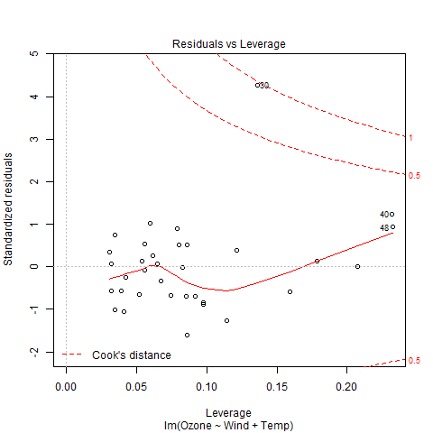
Let us create multiple regression model of airquality dataset present in R base package and plot the model on the graph.

# R program to illustrate
# Multiple Linear Regression
  
# Using airquality dataset
input <- airquality[1:50, 
         c("Ozone", "Wind", "Temp")]
  
# Create regression model
model <- lm(Ozone~Wind + Temp, 
            data = input)
  
# Print the regression model
cat("Regression model:
")
print(model)
  
# Output to be present as PNG file
png(file = "multipleRegGFG.png")
  
# Plot
plot(model)
  
# Save the file.
dev.off()

Выход:

Модель регрессии:
Вызов:
лм (формула = Озон ~ Ветер + Температура, данные = ввод)

Коэффициенты:
(Перехват) Температура ветра  
    -58,239 -0,739 1,329

Логистическая регрессия

Логистическая регрессия - еще один широко используемый метод регрессионного анализа, который предсказывает значение с диапазоном. Кроме того, он используется для прогнозирования значений категориальных данных. Например, электронная почта является либо спамом, либо не спамом, победителем или проигравшим, мужчиной или женщиной и т. Д. Математически,

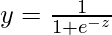
where,
y represents response variable
z represents equation of independent variables or features

Реализация в R

In R programming, glm() function is used to create logistic regression model.

Syntax:
glm(formula, data, family)
Parameters:
formula: represents a formula on the basis of which model has to be fitted
data: represents dataframe on which formula has to be applied
family: represents the type of function to be used. “binomial” for logistic regression

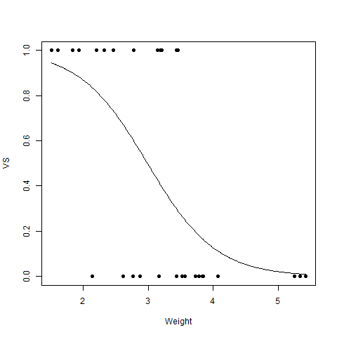
Example:

# R program to illustrate
# Logistic Regression
  
# Using mtcars dataset 
# To create the logistic model
model <- glm(formula = vs ~ wt, 
             family = binomial,
             data = mtcars)
  
# Creating a range of wt values
x <- seq(min(mtcars$wt), 
             max(mtcars$wt), 
             0.01)
  
# Predict using weight
y <- predict(model, list(wt = x), 
             type = "response")
  
# Print model
print(model)
  
# Output to be present as PNG file
png(file = "LogRegGFG.png")
  
# Plot
plot(mtcars$wt, mtcars$vs, pch = 16,
     xlab = "Weight", ylab = "VS")
lines(x, y)
  
# Saving the file
dev.off()

Выход:

Вызов: glm (формула = vs ~ wt, family = binomial, data = mtcars)

Коэффициенты:
(Перехват) вес  
      5,715 -1,911  

Степень свободы: 31 Всего (т. Е. Нулевая); 30 Остаточный
Нулевое отклонение: 43,86 
Остаточное отклонение: 31,37 AIC: 35,37

Picked R язык

Регрессия и ее типы в программировании на R

Типы регрессии

Линейная регрессия

Реализация в R

Множественная регрессия

Реализация в R

Логистическая регрессия

Реализация в R

РЕКОМЕНДУЕМЫЕ СТАТЬИ