Проектирование полосового эллиптического фильтра IIR с использованием Scipy-Python

Опубликовано: 5 Января, 2022

IIR расшифровывается как Infinite Impulse Response, это одна из ярких характеристик многих систем, инвариантных по линейному времени, которые характеризуются наличием импульсной характеристики h (t) / h (n), которая не достигает 0 ни на одном этапе, а вместо этого сохраняется неопределенно долго. .

Что такое полосовой эллиптический фильтр IIR?

Эллиптический фильтр - это особый тип фильтра, который используется в цифровой обработке сигналов, когда требуется быстрый переход от полосы пропускания к полосе заграждения.

Технические характеристики следующие:

Частота полосы пропускания: 1400-2100 Гц
Частота стоп-полосы: 1050-24500 Гц
Пульсация полосы пропускания: 0,4 дБ
Затухание в полосе задерживания: 50 дБ
Частота дискретизации: 7 кГц
Мы построим график амплитуды и фазовой характеристики фильтра.

Пошаговый подход:

Шаг 1: Импорт всех необходимых библиотек.

Python3

 # import required library
 import numpy as np
 import scipy.signal as signal
 import matplotlib.pyplot as plt 

Шаг 2: Определение пользовательских функций mfreqz () и impz () . Mfreqz - это функция для графика амплитуды и фазы, а impz - это функция для импульсной и ступенчатой характеристики].

Python3

# Function to depict magnitude 
# and phase plot
def mfreqz(b, a, Fs):
  
    # Compute frequency response of the
    # filter using signal.freqz function
    wz, hz = signal.freqz(b, a)
  
    # Calculate Magnitude from hz in dB
    Mag = 20*np.log10(abs(hz))
  
    # Calculate phase angle in degree from hz
    Phase = np.unwrap(np.arctan2(np.imag(hz), 
                                 np.real(hz)))*(180/np.pi)
  
    # Calculate frequency in Hz from wz
    Freq = wz*Fs/(2*np.pi)
  
    # Plot filter magnitude and phase responses using subplot.
    fig = plt.figure(figsize=(10, 6))
  
    # Plot Magnitude response
    sub1 = plt.subplot(2, 1, 1)
    sub1.plot(Freq, Mag, "r", linewidth=2)
    sub1.axis([1, Fs/2, -100, 5])
    sub1.set_title("Magnitute Response", fontsize=20)
    sub1.set_xlabel("Frequency [Hz]", fontsize=20)
    sub1.set_ylabel("Magnitude [dB]", fontsize=20)
    sub1.grid()
  
    # Plot phase angle
    sub2 = plt.subplot(2, 1, 2)
    sub2.plot(Freq, Phase, "g", linewidth=2)
    sub2.set_ylabel("Phase (degree)", fontsize=20)
    sub2.set_xlabel(r"Frequency (Hz)", fontsize=20)
    sub2.set_title(r"Phase response", fontsize=20)
    sub2.grid()
  
    plt.subplots_adjust(hspace=0.5)
    fig.tight_layout()
    plt.show()
  
  
# Define impz(b,a) to calculate impulse
# response and step response of a system
# input: b= an array containing numerator
# coefficients,a= an array containing
# denominator coefficients
def impz(b, a):
  
    # Define the impulse sequence of length 60
    impulse = np.repeat(0., 60)
    impulse[0] = 1.
    x = np.arange(0, 60)
  
    # Compute the impulse response
    response = signal.lfilter(b, a, impulse)
  
    # Plot filter impulse and step response:
    fig = plt.figure(figsize=(10, 6))
    plt.subplot(211)
    plt.stem(x, response, "m", use_line_collection=True)
    plt.ylabel("Amplitude", fontsize=15)
    plt.xlabel(r"n (samples)", fontsize=15)
    plt.title(r"Impulse response", fontsize=15)
  
    plt.subplot(212)
    step = np.cumsum(response)
  
    # Compute step response of the system
    plt.stem(x, step, "g", use_line_collection=True)
    plt.ylabel("Amplitude", fontsize=15)
    plt.xlabel(r"n (samples)", fontsize=15)
    plt.title(r"Step response", fontsize=15)
    plt.subplots_adjust(hspace=0.5)
  
    fig.tight_layout()
    plt.show()

Шаг 3: Определите переменные с заданными характеристиками фильтра.

Python3

 # Given specification
 
# Sampling frequency in Hz
 Fs = 7000
 
# Pass band frequency in Hz
 fp = np.array([ 1400 , 2100 ])
 
# Stop band frequency in Hz
 fs = np.array([ 1050 , 2450 ])
 
# Pass band ripple in dB
 Ap = 0.4
 
# Stop band attenuation in dB
 As = 50 

Шаг 4. Вычислите частоту среза

Python3

 # Compute pass band and stop band edge frequencies
 
# Normalized passband edge
 # frequencies wrt Nyquist rate
 wp = fp / (Fs / 2 )
 
# Normalized stopband
 # edge frequencies
 ws = fs / (Fs / 2 ) 

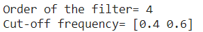
Шаг 5: Вычислить порядок цифрового фильтра Elliptic Bandpass.

Python3

 # Compute order of the elliptic filter
 # using signal.ellipord
 N, wc = signal.ellipord(wp, ws, Ap, As)
 
# Print the order of the filter and
 # cutoff frequencies
 print ( 'Order of the filter=' , N)
 print ( 'Cut-off frequency=' , wc) 

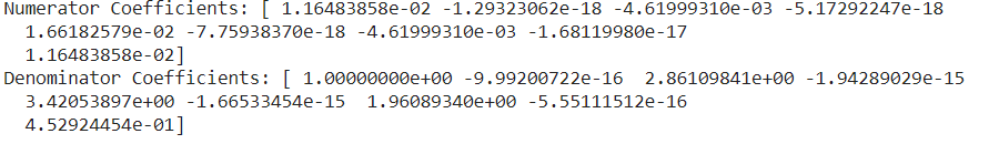
Шаг 6: Разработайте цифровой эллиптический полосовой фильтр.

Python3

 # Design digital elliptic bandpass filter
 # using signal.ellip function
 z, p = signal.ellip(N, Ap, As, wc, 'bandpass' )
 
 
# Print numerator and denomerator
 # coefficients of the filter
 print ( 'Numerator Coefficients:' , z)
 print ( 'Denominator Coefficients:' , p) 

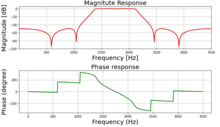
Шаг 7: Постройте график амплитуды и фазовой характеристики.

Python3

 # Depicting visulalizations
 
# Call mfreqz to plot the magnitude and phase response
 mfreqz(z, p, Fs)

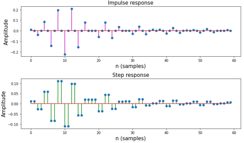
Шаг 8: Постройте импульсную и ступенчатую характеристики фильтра.

Python3

 # Call impz function to plot impulse
 # and step response of the filter
 impz(z, p)

Ниже приведена полная реализация описанного выше пошагового подхода:

Python3

 # Import required library
 import numpy as np
 import scipy.signal as signal
 import matplotlib.pyplot as plt
 
 
# Function to depict magnitude
 # and phase plot
 def mfreqz(b, a, Fs):
 
    # Compute frequency response of the
    # filter using signal.freqz function
    wz, hz = signal.freqz(b, a)
 
    # Calculate Magnitude from hz in dB
    Mag = 20 * np.log10( abs (hz))
 
    # Calculate phase angle in degree from hz
    Phase = np.unwrap(np.arctan2(np.imag(hz),
                                 np.real(hz))) * ( 180 / np.pi)
 
    # Calculate frequency in Hz from wz
    Freq = wz * Fs / ( 2 * np.pi)
 
    # Plot filter magnitude and phase responses using subplot.
    fig = plt.figure(figsize = ( 10 , 6 ))
 
    # Plot Magnitude response
    sub1 = plt.subplot( 2 , 1 , 1 )
    sub1.plot(Freq, Mag, 'r' , linewidth = 2 )
    sub1.axis([ 1 , Fs / 2 , - 100 , 5 ])
    sub1.set_title( 'Magnitute Response' , fontsize = 20 )
    sub1.set_xlabel( 'Frequency [Hz]' , fontsize = 20 )
    sub1.set_ylabel( 'Magnitude [dB]' , fontsize = 20 )
    sub1.grid()
 
    # Plot phase angle
    sub2 = plt.subplot( 2 , 1 , 2 )
    sub2.plot(Freq, Phase, 'g' , linewidth = 2 )
    sub2.set_ylabel( 'Phase (degree)' , fontsize = 20 )
    sub2.set_xlabel(r 'Frequency (Hz)' , fontsize = 20 )
    sub2.set_title(r 'Phase response' , fontsize = 20 )
    sub2.grid()
 
    plt.subplots_adjust(hspace = 0.5 )
    fig.tight_layout()
    plt.show()
 
 
# Define impz(b,a) to calculate impulse
 # response and step response of a system
 # input: b= an array containing numerator
 # coefficients,a= an array containing
 # denominator coefficients
 def impz(b, a):
 
    # Define the impulse sequence of length 60
    impulse = np.repeat( 0. , 60 )
    impulse[ 0 ] = 1.
    x = np.arange( 0 , 60 )
 
    # Compute the impulse response
    response = signal.lfilter(b, a, impulse)
 
    # Plot filter impulse and step response:
    fig = plt.figure(figsize = ( 10 , 6 ))
    plt.subplot( 211 )
    plt.stem(x, response, 'm' , use_line_collection = True )
    plt.ylabel( 'Amplitude' , fontsize = 15 )
    plt.xlabel(r 'n (samples)' , fontsize = 15 )
    plt.title(r 'Impulse response' , fontsize = 15 )
 
    plt.subplot( 212 )
    step = np.cumsum(response)
 
    # Compute step response of the system
    plt.stem(x, step, 'g' , use_line_collection = True )
    plt.ylabel( 'Amplitude' , fontsize = 15 )
    plt.xlabel(r 'n (samples)' , fontsize = 15 )
    plt.title(r 'Step response' , fontsize = 15 )
    plt.subplots_adjust(hspace = 0.5 )
 
    fig.tight_layout()
    plt.show()
 
 
# Given specification
 
# Sampling frequency in Hz
 Fs = 7000
 
# Pass band frequency in Hz
 fp = np.array([ 1400 , 2100 ])
 
# Stop band frequency in Hz
 fs = np.array([ 1050 , 2450 ])
 
# Pass band ripple in dB
 Ap = 0.4
 
# Stop band attenuation in dB
 As = 50
 
# Compute pass band and
 # stop band edge frequencies
 # Normalized passband edge frequencies
 # wrt Nyquist rate
 wp = fp / (Fs / 2 )
 
# Normalized stopband edge frequencies
 ws = fs / (Fs / 2 )
 
# Compute order of the elliptic filter
 # using signal.ellipord
 N, wc = signal.ellipord(wp, ws, Ap, As)
 
# Print the order of the filter and cutoff frequencies
 print ( 'Order of the filter=' , N)
 print ( 'Cut-off frequency=' , wc)
 
# Design digital elliptic bandpass filter
 # using signal.ellip() function
 z, p = signal.ellip(N, Ap, As, wc, 'bandpass' )
 
 
# Print numerator and denomerator coefficients of the filter
 print ( 'Numerator Coefficients:' , z)
 print ( 'Denominator Coefficients:' , p)
 
 
# Depicting visulalizations
 
# Call mfreqz to plot the magnitude and
 # phase response
 mfreqz(z, p, Fs)
 # Call impz function to plot impulse and
 # step response of the filter
 impz(z, p)

Выход:

Внимание компьютерщик! Укрепите свои основы с помощью базового курса программирования Python и изучите основы.

Для начала подготовьтесь к собеседованию. Расширьте свои концепции структур данных с помощью курса Python DS. А чтобы начать свое путешествие по машинному обучению, присоединяйтесь к курсу Машинное обучение - базовый уровень.

Python Статьи Визуализация данных

Проектирование полосового эллиптического фильтра IIR с использованием Scipy-Python

Что такое полосовой эллиптический фильтр IIR?

Технические характеристики следующие:

Пошаговый подход:

Python3

Python3

Python3

Python3

Python3

Python3

Python3

Python3

Python3

РЕКОМЕНДУЕМЫЕ СТАТЬИ