Глубокая нейронная сеть с L - слоями

Эта статья направлена на реализацию глубокой нейронной сети с произвольным количеством скрытых слоев, каждый из которых содержит разное количество нейронов. Мы будем реализовывать эту нейронную сеть, используя несколько вспомогательных функций, и, наконец, мы объединим эти функции, чтобы создать модель нейронной сети L-уровня.

L - слой глубокой структуры нейронной сети (для понимания)

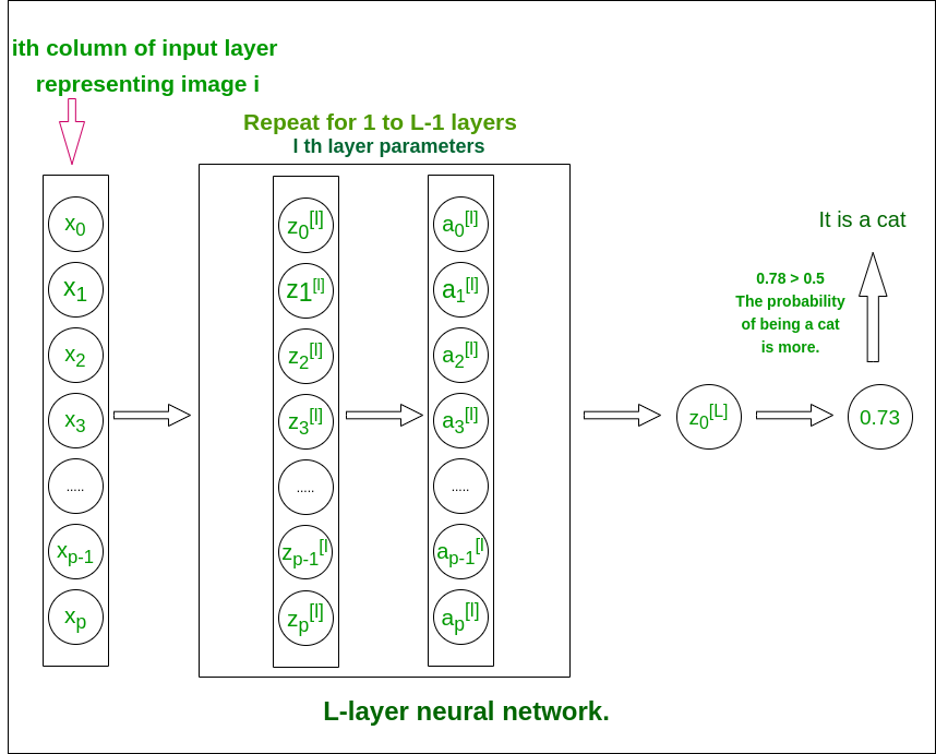
L - слой нейронной сети

Структура модели [LINEAR -> tanh] (L-1 times) -> LINEAR -> SIGMOID. то есть, он имеет слои L-1, использующие функцию гиперболического тангенса в качестве функции активации, за которой следует выходной слой с функцией активации сигмоида.
Подробнее о функциях активации

Пошаговая реализация нейронной сети:

Инициализируйте параметры для L-слоев
Реализуйте модуль прямого распространения
Вычислить потери на последнем слое
Реализуйте модуль обратного распространения
Наконец, обновите параметры
Обучите модель, используя существующий набор обучающих данных
Используйте обученные параметры для тестирования модели

Соглашения об именах, использованные в статье, чтобы избежать путаницы:

• Каждый уровень в сети представлен набором из двух параметров W- матрица (матрица весов) и b- матрица (матрица смещения). Для слоя i эти параметры представлены как Wi и bi соответственно.
• Линейный выход слоя i представлен как Zi , а выходной сигнал после активации представлен как Ai . Размеры Zi и Ai одинаковы.

Размеры матриц весов и смещений.
Входной слой имеет размер (x, m), где m - количество изображений.

Номер слоя	Форма W	Форма b	Линейный выход	Форма активации
Слой 1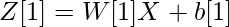
Слой 2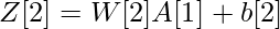
:
Слой L - 1
Слой L

Код: импорт всех необходимых библиотек Python.

Инициализация:

• Мы будем использовать случайную инициализацию для весовых матриц (чтобы избежать идентичного вывода от всех нейронов в одном слое).
• Нулевая инициализация смещений.
• Количество нейронов в каждом слое хранится в словаре layer_dims с ключами в качестве номера слоя.

Код:

Модуль прямого распространения:
Модуль прямого распространения будет завершен в три этапа. В этом порядке мы выполним три функции:

• linear_forward (для вычисления линейного выхода Z для любого слоя)
• linear_activation_forward, где активация будет либо tanh, либо Sigmoid.
• L_model_forward [LINEAR -> tanh] (L-1 раз) -> LINEAR -> SIGMOID (вся модель)

Модуль linear forward (векторизованный по всем примерам) вычисляет следующие уравнения:

Код:

Мы будем использовать эту функцию стоимости, которая будет измерять стоимость выходного слоя для всех данных обучения.

Код:

Модуль обратного распространения:
Подобно модулю прямого распространения, в этом модуле мы также будем реализовывать три функции.

• linear_backward (для вычисления линейного выхода Z для любого слоя)
• linear_activation_backward, где активация будет либо tanh, либо Sigmoid.
• L_model_backward [LINEAR -> tanh] (L-1 раз) -> LINEAR -> SIGMOID (обратное распространение всей модели)

Для слоя i линейная часть: Zi = Wi * A (i - 1) + bi
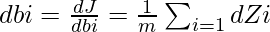
Обозначая dZi = мы можем получить dWi, dbi и dA (i - 1) как -

Код: код Python для реализации

Здесь мы будем вычислять производную сигмоидальных и tanh функций.
Код:

def sigmoid_backward(dA, activation_cache): Z = activation_cache[ 'Z' ] A = sigmoid(Z) return dA * (A * ( 1 - A)) # A*(1 - A) is the derivative of sigmoid function def tanh_backward(dA, activation_cache): Z = activation_cache[ 'Z' ] A = sigmoid(Z) return dA * ( 1 - np.power(A, 2 )) # A*(1 - ) is the derivative of tanh function def linear_activation_backward(dA, cache, activation): linear_cache, activation_cache = cache if activation = = "tanh" : dZ = tanh_backward(dA, activation_cache) dA_prev, dW, db = linear_backward(dZ, linear_cache) elif activation = = "sigmoid" : dZ = sigmoid_backward(dA, activation_cache) dA_prev, dW, db = linear_backward(dZ, linear_cache) return dA_prev, dW, db

L-модель назад:
Напомним, что при реализации функции L_model_forward на каждой итерации вы сохраняли кеш, содержащий (X, W, b и Z). В модуле обратного распространения вы будете использовать эти переменные для вычисления градиентов.

Параметры обновления:

Код: обучение модели

Теперь пришло время собрать все функции, написанные ранее, чтобы сформировать окончательную L-слоистую модель нейронной сети. Аргумент X в L_layer_model будет набором обучающих данных, а Y - соответствующими метками.

Код: реализация функции прогнозирования для проверки предоставленного изображения.

При условии Layers_dims = [12288, 20, 7, 5, 1], когда эта модель обучается с соответствующим количеством обучающих наборов данных, она имеет точность до 80% на тестовых данных.
Параметры находятся после обучения с соответствующим количеством обучающих данных.