Цифровой фильтр Баттерворта низких частот на Python
В этой статье мы собираемся обсудить, как разработать цифровой фильтр Баттерворта низких частот с использованием Python. Фильтр Баттерворта - это тип фильтра обработки сигналов, который имеет как можно более ровную частотную характеристику в полосе пропускания. Давайте возьмем приведенные ниже спецификации, чтобы разработать фильтр и понаблюдать за амплитудой, фазой и импульсной характеристикой цифрового фильтра Баттерворта.
Технические характеристики следующие:
- Частота дискретизации 40 кГц
- Граничная частота полосы пропускания 4 кГц
- Граничная частота полосы задерживания 8 кГц
- Пульсации полосы пропускания 0,5 дБ
- Минимальное затухание в полосе заграждения 40 дБ
Мы построим график амплитуды, фазы и импульсной характеристики фильтра.
Пошаговый подход:
Step 1: Importing all the necessary libraries.
Python3
# import required modulesimport numpy as npimport matplotlib.pyplot as pltfrom scipy import signalimport math |
Step 2: Define variables with the given specifications of the filter.
Python3
# Specifications of Filter # sampling frequencyf_sample = 40000 # pass band frequencyf_pass = 4000 # stop band frequencyf_stop = 8000 # pass band ripplefs = 0.5 # pass band freq in radianwp = f_pass/(f_sample/2) # stop band freq in radianws = f_stop/(f_sample/2) # Sampling TimeTd = 1 # pass band rippleg_pass = 0.5 # stop band attenuationg_stop = 40 |
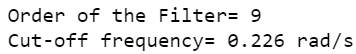
Step3: Building the filter using signal.buttord function.
Python3
# Conversion to prewrapped analog frequencyomega_p = (2/Td)*np.tan(wp/2)omega_s = (2/Td)*np.tan(ws/2) # Design of Filter using signal.buttord functionN, Wn = signal.buttord(omega_p, omega_s, g_pass, g_stop, analog=True) # Printing the values of order & cut-off frequency!print("Order of the Filter=", N) # N is the order# Wn is the cut-off freq of the filterprint("Cut-off frequency= {:.3f} rad/s ".format(Wn)) # Conversion in Z-domain # b is the numerator of the filter & a is the denominatorb, a = signal.butter(N, Wn, "low", True)z, p = signal.bilinear(b, a, fs)# w is the freq in z-domain & h is the magnitude in z-domainw, h = signal.freqz(z, p, 512) |
Выход:
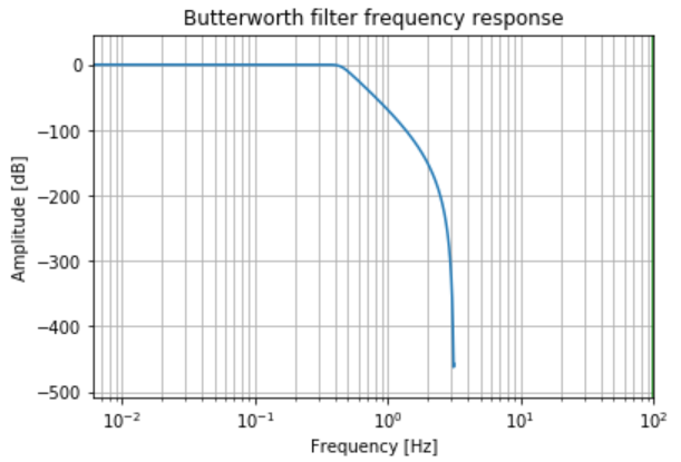
Step 4: Plotting the Magnitude Response.
Python3
# Magnitude Responseplt.semilogx(w, 20*np.log10(abs(h)))plt.xscale("log")plt.title("Butterworth filter frequency response")plt.xlabel("Frequency [Hz]")plt.ylabel("Amplitude [dB]")plt.margins(0, 0.1)plt.grid(which="both", axis="both")plt.axvline(100, color="green")plt.show() |
Выход:
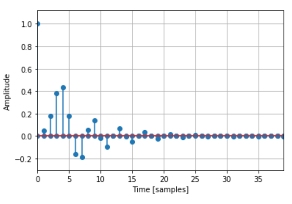
Step 5: Plotting the Impulse Response.
Python3
# Impulse Responseimp = signal.unit_impulse(40)c, d = signal.butter(N, 0.5)response = signal.lfilter(c, d, imp) plt.stem(np.arange(0, 40), imp, use_line_collection=True)plt.stem(np.arange(0, 40), response, use_line_collection=True)plt.margins(0, 0.1) plt.xlabel("Time [samples]")plt.ylabel("Amplitude")plt.grid(True)plt.show() |
Выход:
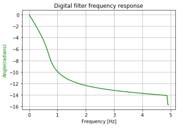
Step 6: Plotting the Phase Response.
Python3
# Phase Responsefig, ax1 = plt.subplots() ax1.set_title("Digital filter frequency response")ax1.set_ylabel("Angle(radians)", color="g")ax1.set_xlabel("Frequency [Hz]") angles = np.unwrap(np.angle(h)) ax1.plot(w/2*np.pi, angles, "g")ax1.grid()ax1.axis("tight")plt.show() |
Выход:
Below is the complete program based on the above approach:
Python
# import required modulesimport numpy as npimport matplotlib.pyplot as pltfrom scipy import signalimport math # Specifications of Filter # sampling frequencyf_sample = 40000 # pass band frequencyf_pass = 4000 # stop band frequencyf_stop = 8000 # pass band ripplefs = 0.5 # pass band freq in radianwp = f_pass/(f_sample/2) # stop band freq in radianws = f_stop/(f_sample/2) # Sampling TimeTd = 1 # pass band rippleg_pass = 0.5 # stop band attenuationg_stop = 40 # Conversion to prewrapped analog frequencyomega_p = (2/Td)*np.tan(wp/2)omega_s = (2/Td)*np.tan(ws/2) # Design of Filter using signal.buttord functionN, Wn = signal.buttord(omega_p, omega_s, g_pass, g_stop, analog=True) # Printing the values of order & cut-off frequency!print("Order of the Filter=", N) # N is the order# Wn is the cut-off freq of the filterprint("Cut-off frequency= {:.3f} rad/s ".format(Wn)) # Conversion in Z-domain # b is the numerator of the filter & a is the denominatorb, a = signal.butter(N, Wn, "low", True)z, p = signal.bilinear(b, a, fs)# w is the freq in z-domain & h is the magnitude in z-domainw, h = signal.freqz(z, p, 512) # Magnitude Responseplt.semilogx(w, 20*np.log10(abs(h)))plt.xscale("log")plt.title("Butterworth filter frequency response")plt.xlabel("Frequency [Hz]")plt.ylabel("Amplitude [dB]")plt.margins(0, 0.1)plt.grid(which="both", axis="both")plt.axvline(100, color="green")plt.show() # Impulse Responseimp = signal.unit_impulse(40)c, d = signal.butter(N, 0.5)response = signal.lfilter(c, d, imp)plt.stem(np.arange(0, 40), imp, use_line_collection=True)plt.stem(np.arange(0, 40), response, use_line_collection=True)plt.margins(0, 0.1)plt.xlabel("Time [samples]")plt.ylabel("Amplitude")plt.grid(True)plt.show() # Phase Responsefig, ax1 = plt.subplots()ax1.set_title("Digital filter frequency response")ax1.set_ylabel("Angle(radians)", color="g")ax1.set_xlabel("Frequency [Hz]")angles = np.unwrap(np.angle(h))ax1.plot(w/2*np.pi, angles, "g")ax1.grid()ax1.axis("tight")plt.show() |
Выход:
Внимание компьютерщик! Укрепите свои основы с помощью базового курса программирования Python и изучите основы.
Для начала подготовьтесь к собеседованию. Расширьте свои концепции структур данных с помощью курса Python DS. А чтобы начать свое путешествие по машинному обучению, присоединяйтесь к курсу Машинное обучение - базовый уровень.