Seaborn Kdeplot - подробное руководство

График оценки плотности ядра (KDE) и график Kdeplot позволяют нам оценить функцию плотности вероятности непрерывного или непараметрического из нашей кривой набора данных в одном или нескольких измерениях, это означает, что мы можем создать один график для нескольких выборок, который помогает в большем количестве эффективная визуализация данных.

Чтобы использовать модуль Seaborn, нам необходимо установить модуль, используя следующую команду:

 pip install seaborn

Syntax: seaborn.kdeplot(x=None, *, y=None, vertical=False, palette=None, **kwargs)

Parameters:

x, y : vectors or keys in data

vertical : boolean (True or False)

data : pandas.DataFrame, numpy.ndarray, mapping, or sequence

Мы изучаем использование некоторых параметров на некоторых конкретных примерах:

First import the corresponding library

Draw a simple one-dimensional kde image:

Let’s see the Kde of our variable x-axis and y-axis, so let pass the x variable into the kdeplot() methods.

Выход:

Then after check for y-axis.

Выход:

Используйте Shade, чтобы заполнить область, покрытую кривой:

We can highlight the plot using shade to the area covered by the curve. If True, shadow processing is performed in the area below the kde curve, and color controls the color of the curve and shadow

Выход:

You can change the Shade color with color attributes:

Выход:

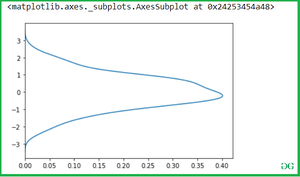
Use Vertical to draw indicates whether to draw on the X axis or on the Y axis

Выход:

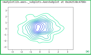
Двумерный график Kdeplot для двух переменных:

Simple pass the two variables into the seaborn.kdeplot() methods.

Выход:

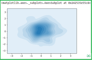
Shade the area covered by a curve with shade attributes:

Выход:

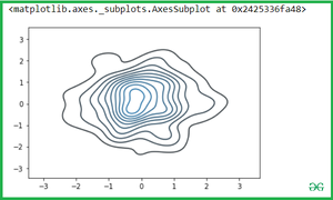
Now you can change the color with cmap attributes:

Выход:

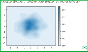
Use of Cbar: If True, add a colorbar to annotate the color mapping in a bivariate plot. Note: Does not currently support plots with a hue variable well.

Выход:

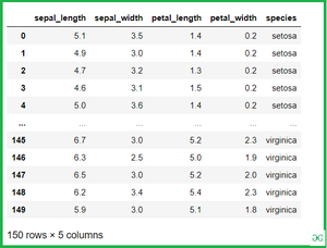
Давайте посмотрим на пример с набором данных Iris, который представляет собой график распределения для каждого столбца набора данных широкой формы:

Набор данных ирисов состоит из трех разных типов ирисов (Setosa, Versicolour и Virginica), длина лепестков и чашелистиков, хранящихся в numpy.ndarray размером 150 × 4.

Loading the iris dataset for Kdeplot:

Выход:

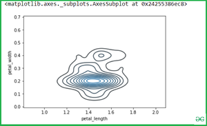
Двумерный график Kdeplot для двух переменных радужной оболочки:

Once we have species set then if we want to simply calculate the petal_length and petal_width then Simple pass the two variables(Setosa and verginica ) into the seaborn.kdeplot() methods.

Выход:

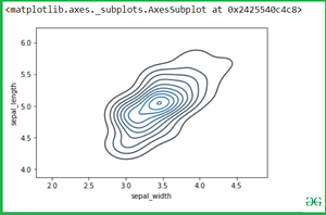
See another example if we want to calculate another variable attribute which is sepal_width and sepal_length.

Выход:

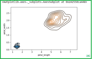
If we pass the two separate Kdeplot with different variable:

Выход:

Внимание компьютерщик! Укрепите свои основы с помощью базового курса программирования Python и изучите основы.

Для начала подготовьтесь к собеседованию. Расширьте свои концепции структур данных с помощью курса Python DS. А чтобы начать свое путешествие по машинному обучению, присоединяйтесь к курсу Машинное обучение - базовый уровень.