Построение трехмерной поверхности в Python с использованием Matplotlib
График поверхности - это представление трехмерного набора данных. Он описывает функциональную взаимосвязь между двумя независимыми переменными X и Z и обозначенной зависимой переменной Y, а не показывает отдельные точки данных. Это сопутствующий участок контурного участка. Это похоже на каркасный график, но каждая грань каркаса представляет собой заполненный многоугольник. Это помогает создать топологию визуализируемой поверхности.
Создание 3D-графика поверхности
The axes3d present in Matplotlib’s mpl_toolkits.mplot3d toolkit provides the necessary functions used to create 3D surface plots.Surface plots are created by using ax.plot_surface() function.
Синтаксис:
ax.plot_surface (X, Y, Z)
where X and Y are 2D array of points of x and y while Z is 2D array of heights.Some more attributes of ax.plot_surface() function are listed below:
| Attribute | Description |
|---|---|
| X, Y, Z | 2D arrays of data values |
| cstride | array of column stride(step size) |
| rstride | array of row stride(step size) |
| ccount | number of colums to be used, default is 50 |
| rcount | number of row to be used, default is 50 |
| color | color of the surface |
| cmap | colormap for the surface |
| norm | instance to normalize values of color map |
| vmin | minimum value of map |
| vmax | maximum value of map |
| facecolors | face color of individual surface |
| shade | shades the face color |
Пример: давайте создадим трехмерную поверхность, используя указанную выше функцию.
# Import librariesfrom mpl_toolkits import mplot3dimport numpy as npimport matplotlib.pyplot as plt # Creating datasetx = np.outer(np.linspace(-3, 3, 32), np.ones(32))y = x.copy().T # transposez = (np.sin(x **2) + np.cos(y **2) ) # Creating figyrefig = plt.figure(figsize =(14, 9))ax = plt.axes(projection ="3d") # Creating plotax.plot_surface(x, y, z) # show plotplt.show() |
Выход: 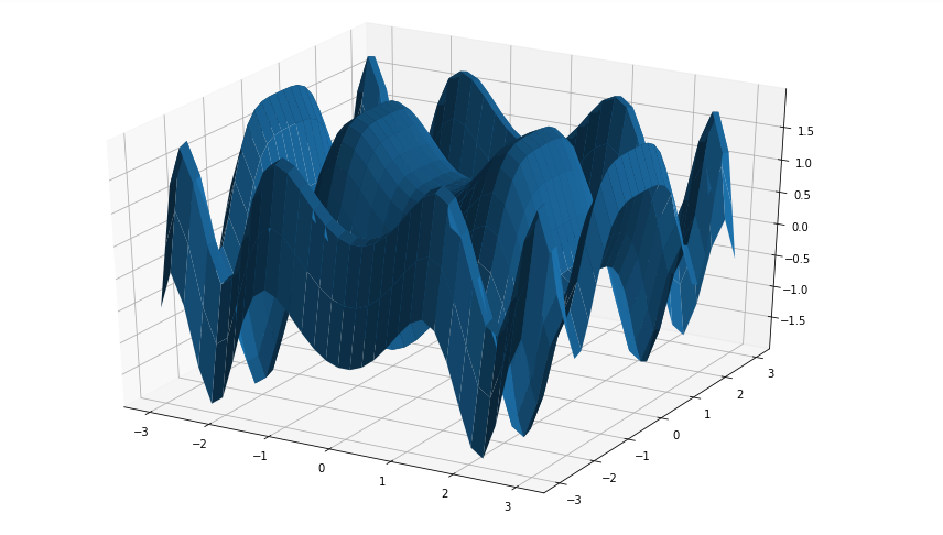
Градиентная поверхность
Градиентный график поверхности представляет собой комбинацию трехмерного графика поверхности с двухмерным контурным графиком. На этом графике трехмерная поверхность окрашена как двухмерный контурный график. Детали, расположенные высоко на поверхности, имеют другой цвет, чем детали, расположенные низко на поверхности.
Синтаксис:
surf = ax.plot_surface(X, Y, Z, cmap=, linewidth=0, antialiased=False)
The attribute cmap= stes the color of the surface. A color bar can also be added by calling fig.colorbar. The code below create a gradient surface plot:
Example:
# Import librariesfrom mpl_toolkits import mplot3dimport numpy as npimport matplotlib.pyplot as plt # Creating datasetx = np.outer(np.linspace(-3, 3, 32), np.ones(32))y = x.copy().T # transposez = (np.sin(x **2) + np.cos(y **2) ) # Creating figyrefig = plt.figure(figsize =(14, 9))ax = plt.axes(projection ="3d") # Creating color mapmy_cmap = plt.get_cmap("hot") # Creating plotsurf = ax.plot_surface(x, y, z, cmap = my_cmap, edgecolor ="none") fig.colorbar(surf, ax = ax, shrink = 0.5, aspect = 5) ax.set_title("Surface plot") # show plotplt.show() |
Выход: 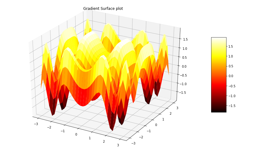
Трехмерный поверхностный график с двухмерными проекциями контурных графиков
Графики 3D-поверхности, построенные с помощью Matplotlib, можно проецировать на 2D-поверхности. Приведенный ниже код создает 3D-графики и визуализирует их проекцию на 2D-контурном графике:
Example:
# Import librariesfrom mpl_toolkits import mplot3dimport numpy as npimport matplotlib.pyplot as plt # Creating datasetx = np.outer(np.linspace(-3, 3, 32), np.ones(32))y = x.copy().T # transposez = (np.sin(x **2) + np.cos(y **2) ) # Creating figyrefig = plt.figure(figsize =(14, 9))ax = plt.axes(projection ="3d") # Creating color mapmy_cmap = plt.get_cmap("hot") # Creating plotsurf = ax.plot_surface(x, y, z, rstride = 8, cstride = 8, alpha = 0.8, cmap = my_cmap)cset = ax.contourf(x, y, z, zdir ="z", offset = np.min(z), cmap = my_cmap)cset = ax.contourf(x, y, z, zdir ="x", offset =-5, cmap = my_cmap)cset = ax.contourf(x, y, z, zdir ="y", offset = 5, cmap = my_cmap)fig.colorbar(surf, ax = ax, shrink = 0.5, aspect = 5) # Adding labelsax.set_xlabel("X-axis")ax.set_xlim(-5, 5)ax.set_ylabel("Y-axis")ax.set_ylim(-5, 5)ax.set_zlabel("Z-axis")ax.set_zlim(np.min(z), np.max(z))ax.set_title("3D surface having 2D contour plot projections") # show plotplt.show() |
Выход: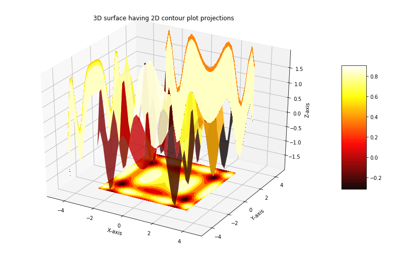
Внимание компьютерщик! Укрепите свои основы с помощью базового курса программирования Python и изучите основы.
Для начала подготовьтесь к собеседованию. Расширьте свои концепции структур данных с помощью курса Python DS. А чтобы начать свое путешествие по машинному обучению, присоединяйтесь к курсу Машинное обучение - базовый уровень.