Python - основы Pandas с использованием набора данных Iris

Опубликовано: 27 Марта, 2022

Язык Python - один из самых популярных языков программирования, поскольку он динамичен по сравнению с другими. Python - это простой высокоуровневый язык с открытым исходным кодом, используемый для программирования общего назначения. В нем много библиотек с открытым исходным кодом, и Pandas - одна из них. Pandas - это мощная, быстрая и гибкая библиотека с открытым исходным кодом, используемая для анализа данных и манипуляций с фреймами данных / наборами данных. Pandas можно использовать для чтения и записи данных в наборе данных различных форматов, таких как CSV (значения, разделенные запятыми), txt, xls (Microsoft Excel) и т. Д.
В этом посте вы узнаете о различных функциях Pandas в Python и о том, как использовать их на практике.

Предварительные требования: Базовые знания о программировании на Python.

Установка:

Итак, если вы новичок в использовании Pandas, сначала вам следует установить Pandas в своей системе.
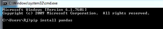
Перейдите в командную строку и запустите ее от имени администратора. Убедитесь, что вы подключены к Интернету, чтобы загрузить и установить его в своей системе.

Затем введите « pip install pandas » и нажмите клавишу Enter.

Загрузите набор данных «Iris.csv» отсюда.

Набор данных Iris - это Hello World для науки о данных, поэтому, если вы начали свою карьеру в области науки о данных и машинного обучения, вы будете практиковать базовые алгоритмы машинного обучения на этом знаменитом наборе данных. Набор данных радужки содержит пять столбцов, таких как длина лепестка, ширина лепестка, длина чашелистика, ширина чашелистника и тип вида.
Ирис - это цветущее растение, исследователи измерили различные характеристики разных цветов ириса и записали их в цифровом виде.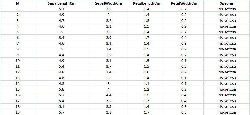

Getting Started with Pandas:

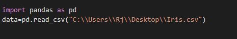
Code: Importing pandas to use in our code as pd.

import pandas as pd

Code: Reading the dataset “Iris.csv”.

data = pd.read_csv("your downloaded dataset location ")

Code: Displaying up the top rows of the dataset with their columns
The function head() will display the top rows of the dataset, the default value of this function is 5, that is it will show top 5 rows when no argument is given to it.

data.head()

Output: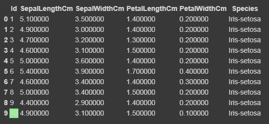

Displaying the number of rows randomly.
In sample() function, it will also display the rows according to arguments given, but it will display the rows randomly.

data.sample(10)

Output: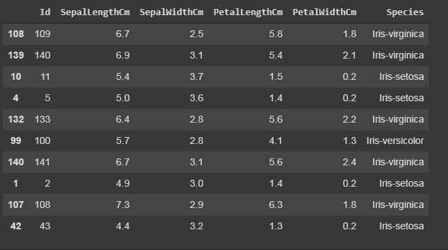

Code: Displaying the number of columns and names of the columns.
The column() function prints all the columns of the dataset in a list form.

data.columns

Output: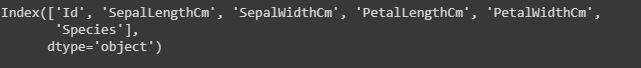

Code: Displaying the shape of the dataset.
The shape of the dataset means to print the total number of rows or entries and the total number of columns or features of that particular dataset.

#The first one is the number of rows and 
# the other one is the number of columns.
data.shape

Output: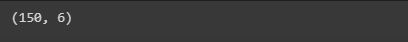

Code: Display the whole dataset

print(data)

Output: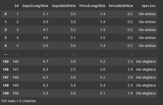

Code: Slicing the rows.
Slicing means if you want to print or work upon a particular group of lines that is from 10th row to 20th row.

#data[start:end]
#start is inclusive whereas end is exclusive
print(data[10:21])
# it will print the rows from 10 to 20.
  
# you can also save it in a variable for further use in analysis
sliced_data=data[10:21]
print(sliced_data)

Output: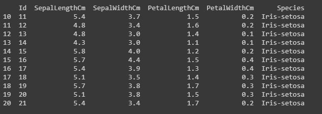

Code: Displaying only specific columns.
In any dataset, it is sometimes needed to work upon only specific features or columns, so we can do this by the following code.

#here in the case of Iris dataset
#we will save it in a another variable named "specific_data"
  
specific_data=data[["Id","Species"]]
#data[["column_name1","column_name2","column_name3"]]
  
#now we will print the first 10 columns of the specific_data dataframe.
print(specific_data.head(10))

Output: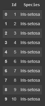

Filtering:Displaying the specific rows using “iloc” and “loc” functions.

The “loc” functions use the index name of the row to display the particular row of the dataset.
The “iloc” functions use the index integer of the row, which gives complete information about the row.
Code:

#here we will use iloc
  
data.iloc[5]
#it will display records only with species "Iris-setosa".
data.loc[data["Species"] == "Iris-setosa"]

Output: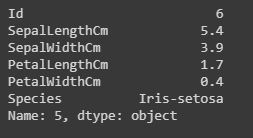
iloc()[/caption]

loc()

Code: Counting the number of counts of unique values using “value_counts()”.
The value_counts() function, counts the number of times a particular instance or data has occurred.

#In this dataset we will work on the Species column, it will count number of times a particular species has occurred.
data["Species"].value_counts()
#it will display in descending order.

Output: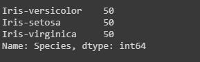

Calculating sum, mean and mode of a particular column.
We can also calculate the sum, mean and mode of any integer columns as I have done in the following code.

# data["column_name"].sum()
  
sum_data = data["SepalLengthCm"].sum()
mean_data = data["SepalLengthCm"].mean()
median_data = data["SepalLengthCm"].median()
  
print("Sum:",sum_data, "
Mean:", mean_data, "
Median:",median_data)

Output: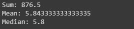

Code: Extracting minimum and maximum from a column.
Identifying minimum and maximum integer, from a particular column or row can also be done in a dataset.

min_data=data["SepalLengthCm"].min()
max_data=data["SepalLengthCm"].max()
  
print("Minimum:",min_data, "
Maximum:", max_data)

Output: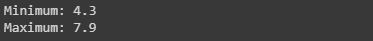

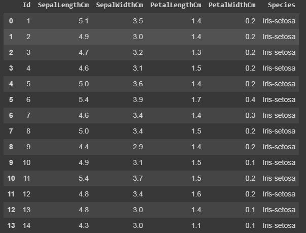
Code: Adding a column to the dataset.
If want to add a new column in our dataset, as we are doing any calculations or extracting some information from the dataset, and if you want to save it a new column. This can be done by the following code by taking a case where we have added all integer values of all columns.

# For example, if we want to add a column let say "total_values", 
# that means if you want to add all the integer value of that particular
# row and get total answer in the new column "total_values".
# first we will extract the columns which have integer values.
cols = data.columns
  
# it will print the list of column names.
print(cols)
  
# we will take that columns which have integer values.
cols = cols[1:5]
  
# we will save it in the new dataframe variable
data1 = data[cols]
  
# now adding new column "total_values" to dataframe data.
data["total_values"]=data1[cols].sum(axis=1)
  
# here axis=1 means you are working in rows, 
# whereas axis=0 means you are working in columns.

Output: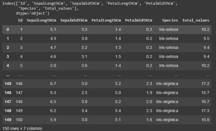

Code: Renaming the columns.
Renaming our column names can also be possible in python pandas libraries. We have used the rename() function, where we have created a dictionary “newcols” to update our new column names. The following code illustrates that.

newcols={
"Id":"id",
"SepalLengthCm":"sepallength"
"SepalWidthCm":"sepalwidth"}
  
data.rename(columns=newcols,inplace=True)
  
print(data.head())

Output: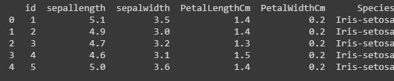

Formatting and Styling:
Conditional formatting can be applied to your dataframe by using Dataframe.style function. Styling is used to visualize your data, and most convenient way of visualizing your dataset is in tabular form.
Here we will highlight the minimum and maximum from each row and columns.

#this is an example of rendering a datagram, 
which is not visualised by any styles. 
data.style

Output: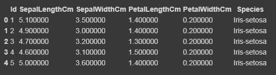

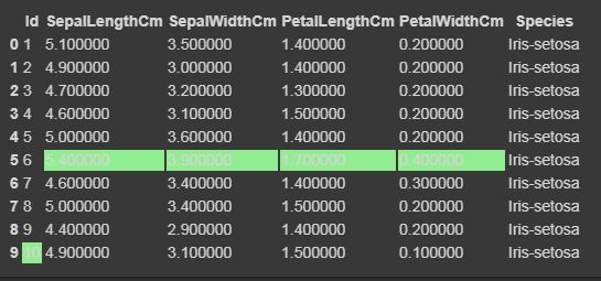
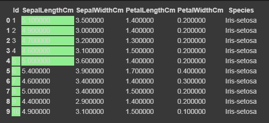
Now we will highlight the maximum and minimum column-wise, row-wise, and the whole dataframe wise using Styler.apply function. The Styler.apply function passes each column or row of the dataframe depending upon the keyword argument axis. For column-wise use axis=0, row-wise use axis=1, and for the entire table at once use axis=None.

# we will here print only the top 10 rows of the dataset, 
# if you want to see the result of the whole dataset remove 
#.head(10) from the below code
  
data.head(10).style.highlight_max(color="lightgreen", axis=0)
  
data.head(10).style.highlight_max(color="lightgreen", axis=1)
  
data.head(10).style.highlight_max(color="lightgreen", axis=None)

Output:

for axis=0

for axis=1

for axis=None

Code: Cleaning and detecting missing values
In this dataset, we will now try to find the missing values i.e NaN, which can occur due to several reasons.

data.isnull()
#if there is data is missing, it will display True else False.

Output:

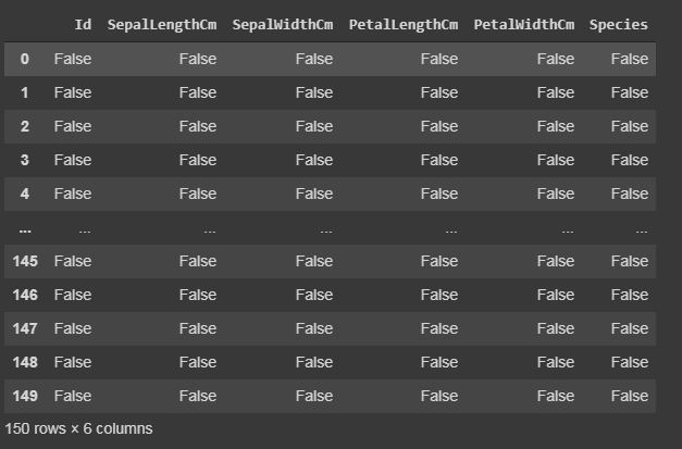
isnull()

Code: Summarizing the missing values.
We will display how many missing values are present in each column.

data.isnull.sum()

Output: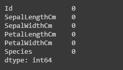

Heatmap: Importing seaborn
The heatmap is a data visualisation technique which is used to analyse the dataset as colors in two dimensions. Basically it shows correlation between all numerical variables in the dataset. Heatmap is an attribute of the Seaborn library.
Code:

import seaborn as sns
  
iris = sns.load_dataset("iris")
sns.heatmap(iris.corr(),camp = "YlGnBu", linecolor = "white", linewidths = 1)

Output: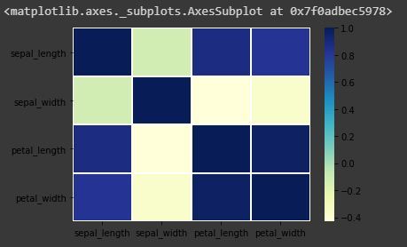

Code: Annotate each cell with the numeric value using integer formatting

sns.heatmap(iris.corr(),camp = "YlGnBu", linecolor = "white", linewidths = 1, annot = True )

Output:

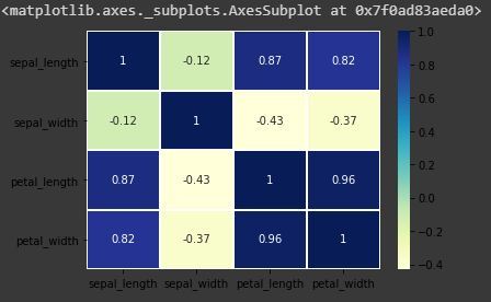
heatmap with annot=True

Pandas Dataframe Correlation:
Pandas correlation is used to determine pairwise correlation of all the columns of the dataset. In datafram.corr(), the missing values are excluded and non-numeric columns are also ignored.
Code:

data.corr(method="pearson")

Output:

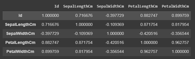
data.corr()

The output dataframe can be seen as for any cell, row variable correlation with the column variable is the value of the cell. The correlation of a variable with itself is 1. For that reason, all the diagonal values are 1.00.

Multivariate Analysis:
Pair plot is used to visualize the relationship between each type of column variable. It is implemented only by one line code, which is as follows :
Code:

g = sns.pairplot(data,hue="Species")

Output:

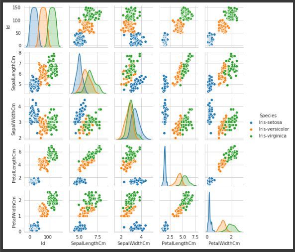
Pairplot of variable “Species”, to make it more understandable.

Attention geek! Strengthen your foundations with the Python Programming Foundation Course and learn the basics.

To begin with, your interview preparations Enhance your Data Structures concepts with the Python DS Course. And to begin with your Machine Learning Journey, join the Machine Learning – Basic Level Course

Python - основы Pandas с использованием набора данных Iris

РЕКОМЕНДУЕМЫЕ СТАТЬИ