Обычный метод наименьших квадратов (OLS) с использованием статистических моделей

Опубликовано: 30 Ноября, 2021

В этой статье мы будем использовать модуль statsmodels Python для реализации метода линейной регрессии с обычными наименьшими квадратами ( OLS).

Вступление :
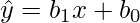
Модель линейной регрессии устанавливает связь между зависимой переменной ( y ) и по крайней мере одной независимой переменной ( x ) как:

В методе OLS мы должны выбрать значения

а также

таким образом, чтобы минимизировать общую сумму квадратов разницы между вычисленными и наблюдаемыми значениями y.
Формула для OLS:

Где,
= прогнозируемое значение для i-го наблюдения
= фактическое значение для i-го наблюдения
= ошибка / невязка для i-го наблюдения
n = общее количество наблюдений

Чтобы получить значения а также которые минимизируют S, мы можем взять частную производную для каждого коэффициента и приравнять ее к нулю.

Modules used :

statsmodels : provides classes and functions for the estimation of many different statistical models.
```
pip install statsmodels
```
pandas : library used for data manipulation and analysis.
```
pip install pandas
```
NumPy : core library for array computing.
```
pip install numpy
```
Matplotlib : a comprehensive library used for creating static and interactive graphs and visualisations.
```
pip install matplotlib
```

Approach :

First we define the variables x and y. In the example below, the variables are read from a csv file using pandas. The file used in the example can be downloaded here.
Next, We need to add the constant to the equation using the add_constant() method.
The OLS() function of the statsmodels.api module is used to perform OLS regression. It returns an OLS object. Then fit() method is called on this object for fitting the regression line to the data.
The summary() method is used to obtain a table which gives an extensive description about the regression results

Syntax : statsmodels.api.OLS(y, x)
Parameters :
y : the variable which is dependent on x
x : the independent variable

Code:

import statsmodels.api as sm
import pandas as pd
  
# reading data from the csv
data = pd.read_csv("train.csv")
  
# defining the variables
x = data["x"].tolist()
y = data["y"].tolist()
  
# adding the constant term
x = sm.add_constant(x)
  
# performing the regression
# and fitting the model
result = sm.OLS(y, x).fit()
  
# printing the summary table
print(result.summary())

Output :

                            OLS Regression Results                            
==============================================================================
Dep. Variable:                      y   R-squared:                       0.989
Model:                            OLS   Adj. R-squared:                  0.989
Method:                 Least Squares   F-statistic:                 2.709e+04
Date:                Fri, 26 Jun 2020   Prob (F-statistic):          1.33e-294
Time:                        15:55:38   Log-Likelihood:                -757.98
No. Observations:                 300   AIC:                             1520.
Df Residuals:                     298   BIC:                             1527.
Df Model:                           1                                         
Covariance Type:            nonrobust                                         
==============================================================================
                 coef    std err          t      P>|t|      [0.025      0.975]
------------------------------------------------------------------------------
const         -0.4618      0.360     -1.284      0.200      -1.169       0.246
x1             1.0143      0.006    164.598      0.000       1.002       1.026
==============================================================================
Omnibus:                        1.034   Durbin-Watson:                   2.006
Prob(Omnibus):                  0.596   Jarque-Bera (JB):                0.825
Skew:                           0.117   Prob(JB):                        0.662
Kurtosis:                       3.104   Cond. No.                         120.
==============================================================================

Warnings:
[1] Standard Errors assume that the covariance matrix of the errors is correctly specified.

Description of some of the terms in the table :

R-squared : the coefficient of determination. It is the proportion of the variance in the dependent variable that is predictable/explained
Adj. R-squared : Adjusted R-squared is the modified form of R-squared adjusted for the number of independent variables in the model. Value of adj. R-squared increases, when we include extra variables which actually improve the model.
F-statistic : the ratio of mean squared error of the model to the mean squared error of residuals. It determines the overall significance of the model.
coef : the coefficients of the independent variables and the constant term in the equation.
t : the value of t-statistic. It is the ratio of the difference between the estimated and hypothesised value of a parameter, to the standard error

Predicting values:
From the results table, we note the coefficient of x and the constant term. These values are substituted in the original equation and the regression line is plotted using matplotlib.
Code:

import pandas as pd
import matplotlib.pyplot as plt
import numpy as np
  
# reading data from the csv
data = pd.read_csv("train.csv")
  
# plotting the original values
x = data["x"].tolist()
y = data["y"].tolist()
plt.scatter(x, y)
  
# finding the maximum and minimum
# values of x, to get the
# range of data
max_x = data["x"].max()
min_x = data["x"].min()
  
# range of values for plotting
# the regression line
x = np.arange(min_x, max_x, 1)
  
# the substituted equation
y = 1.0143 * x - 0.4618
  
# plotting the regression line
plt.plot(y, "r")
plt.show()

Output:

Attention geek! Strengthen your foundations with the Python Programming Foundation Course and learn the basics.

To begin with, your interview preparations Enhance your Data Structures concepts with the Python DS Course. And to begin with your Machine Learning Journey, join the Machine Learning – Basic Level Course

Python Наука о данных

Обычный метод наименьших квадратов (OLS) с использованием статистических моделей

РЕКОМЕНДУЕМЫЕ СТАТЬИ